library(dplyr)
#>
#> Attaching package: 'dplyr'
#> The following objects are masked from 'package:stats':
#>
#>     filter, lag
#> The following objects are masked from 'package:base':
#>
#>     intersect, setdiff, setequal, union
library(ggplot2)
library(survival)
library(survParamSim)

set.seed(12345)
The goal of survParamSim is to perform survival simulation with parametric survival model generated from ‘survreg’ function in ‘survival’ package. In each simulation, coefficients are resampled from variance-covariance matrix of parameter estimates, in order to capture uncertainty in model parameters.
Fit model with survreg() function
Before running a parametric survival simulation, you need to fit a
model to your data using survreg() function of
survival package.
In this vignette, we will be using colon dataset available
in survival package, where the treatment effect of adjuvant
Levamisole+5-FU for colon cancer over placebo is evaluated.
First, we load the data and do some data wrangling.
# ref for dataset https://vincentarelbundock.github.io/Rdatasets/doc/survival/colon.html
colon2 <-
  as_tibble(colon) %>%
  # recurrence only and not including Lev alone arm
  filter(rx != "Lev",
         etype == 1) %>%
  # Same definition as Lin et al, 1994
  mutate(rx = factor(rx, levels = c("Obs", "Lev+5FU")),
         depth = as.numeric(extent <= 2))
Shown below are Kaplan-Meier curves for visually checking the
data.
The second plot is looking at how many censoring we have over
time.
Looks like we have a fairly uniform censoring between 1800 to 3000 days
- this is attributable to a steady clinical study enrollment.
survfit.colon <- survfit(Surv(time, status) ~ rx, data = colon2)
survminer::ggsurvplot(survfit.colon)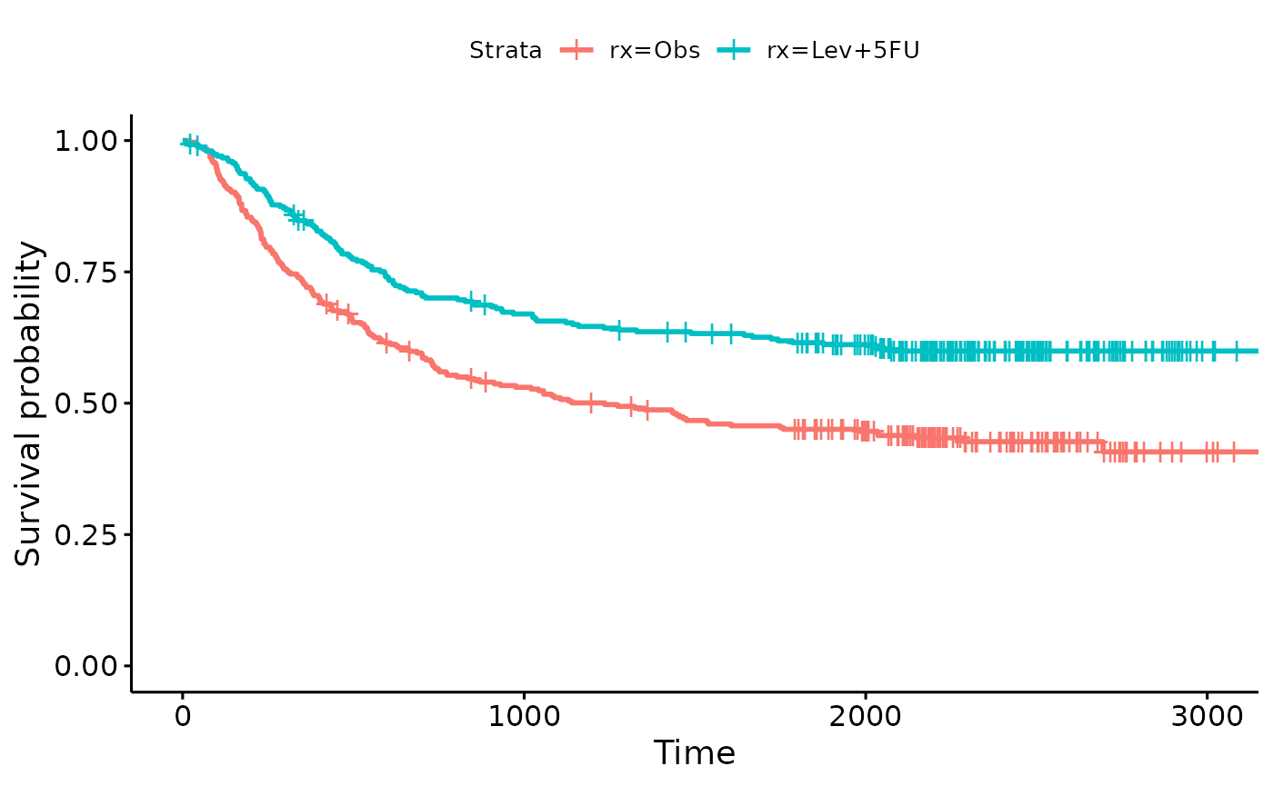
survfit.colon.censor <- survfit(Surv(time, 1-status) ~ rx, data = colon2)
survminer::ggsurvplot(survfit.colon.censor)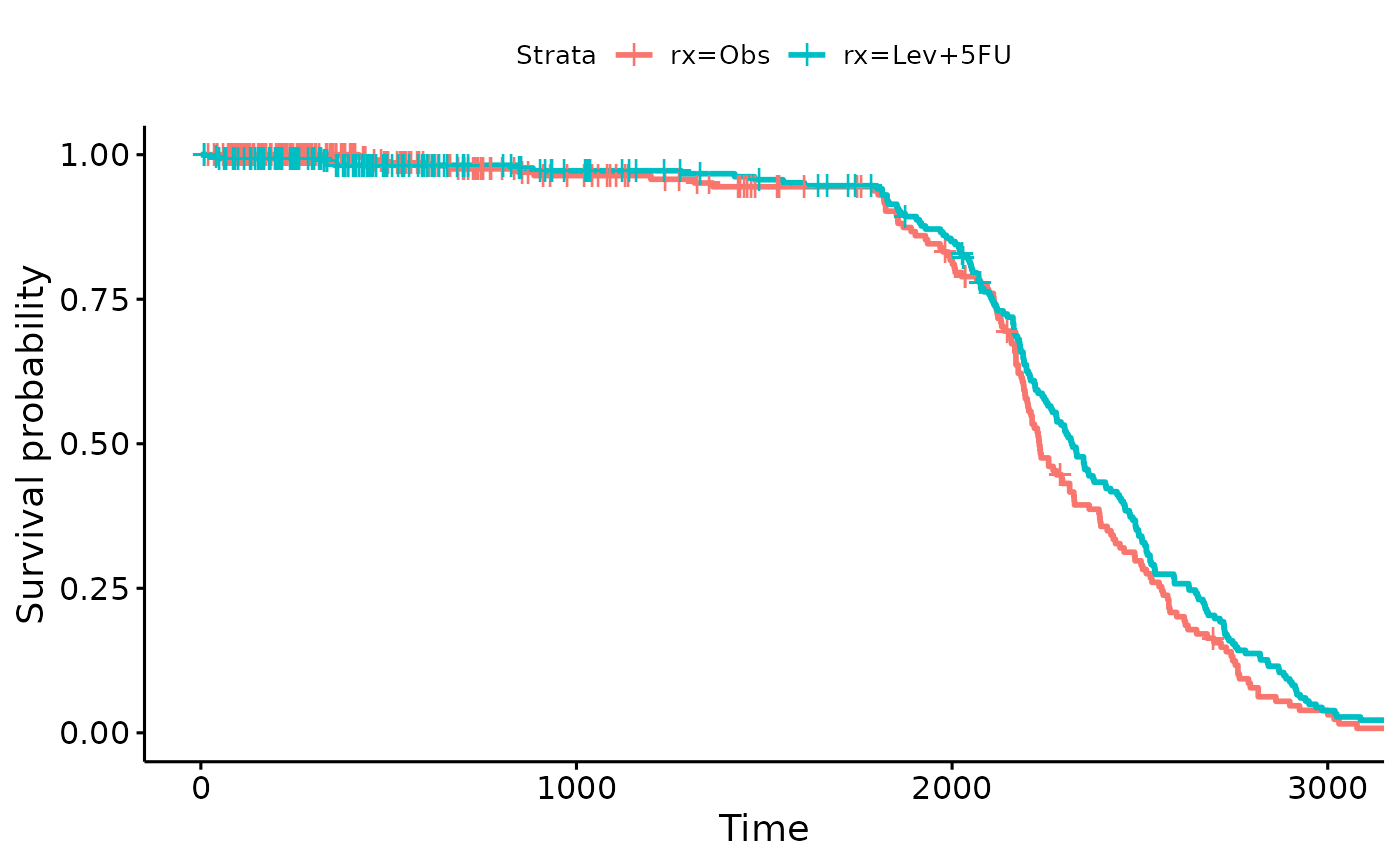
Next we fit a lognormal parametric model for the data.
Here we are using node4 and depth as
additional covariates in addition to treatment (rx).
You can see that all of the factor has strong association with the
outcome.
fit.colon <- survreg(Surv(time, status) ~ rx + node4 + depth,
                     data = colon2, dist = "lognormal")

summary(fit.colon)
#>
#> Call:
#> survreg(formula = Surv(time, status) ~ rx + node4 + depth, data = colon2,
#>     dist = "lognormal")
#>               Value Std. Error     z       p
#> (Intercept)  7.5103     0.1343 55.92 < 2e-16
#> rxLev+5FU    0.7606     0.1677  4.54 5.7e-06
#> node4       -1.3474     0.1816 -7.42 1.2e-13
#> depth        1.1243     0.2661  4.22 2.4e-05
#> Log(scale)   0.6040     0.0461 13.10 < 2e-16
#>
#> Scale= 1.83
#>
#> Log Normal distribution
#> Loglik(model)= -2561.7   Loglik(intercept only)= -2607.6
#>  Chisq= 91.8 on 3 degrees of freedom, p= 9e-20
#> Number of Newton-Raphson Iterations: 4
#> n= 619
Perform simulation
surv_param_sim() is the main function of the package
that takes survreg object as described above.
It also require you to supply newdata, which is required
even if it is not new - i.e. the same data was used for both
survreg() and surv_param_sim().
What it does is: 1. Re-sample all the coefficients in the parametric
survival model from variance-covariance matrix for n.rep
times. 2. Perform survival time for all subjects in newdata
with the corresponding covariates, using one of the resampled
coefficients. Also generate censoring time according to
censor.dur (if not NULL), and replace the simulated
survival time above if censoring time is earlier. 4. Repeat the steps 2.
for n.rep times.
sim <-
  surv_param_sim(object = fit.colon, newdata = colon2,
                 # Simulate censoring according to the plot above
                 censor.dur = c(1800, 3000),
                 # Simulate only 100 times to make the example go fast
                 n.rep = 100)
After the simulation is performed, you can either extract raw
simulation results or further calculate Kaplan-Meier estimates or hazard
ratio of treatment effect, as you see when you type sim in
the console.
sim
#> ---- Simulated survival data with the following model ----
#> survreg(formula = Surv(time, status) ~ rx + node4 + depth, data = colon2,
#>     dist = "lognormal")
#>
#> * Use `extract_sim()` function to extract individual simulated survivals
#> * Use `calc_km_pi()` function to get survival curves and median survival time
#> * Use `calc_hr_pi()` function to get hazard ratio
#>
#> * Settings:
#>     #simulations: 100
#>     #subjects: 619 (without NA in model variables)
Survival time profile
To calculate survival curves for each simulated dataset,
calc_ave_km_pi() or calc_km_pi() can be used
on the simulated object above.
km.pi <- calc_km_pi(sim, trt = "rx")
#> Warning in calc_km_pi(sim, trt = "rx"): 70 of 200 simulations (#rep * #trt *
#> #group) did not reach median survival time and these are not included for
#> prediction interval calculation. You may want to delay the `censor.dur` in
#> simulation.
km.pi
#> ---- Simulated and observed (if calculated) survival curves ----
#> * Use `extract_medsurv_pi()` to extract prediction intervals of median survival times
#> * Use `extract_km_pi()` to extract prediction intervals of K-M curves
#> * Use `plot_km_pi()` to draw survival curves
#>
#> * Settings:
#>     trt: rx
#>     group: NA
#>     pi.range: 0.95
#>     calc.obs: TRUE
#>     method: K-M on simulated survival using `calc_km_pi()`
Similar to the raw simulated object, you can have a few options for
further processing - one of them is plotting prediction intervals with
plot_km_pi() function.
plot_km_pi(km.pi) +
  theme(legend.position = "bottom") +
  labs(y = "Recurrence free rate") +
  expand_limits(y = 0)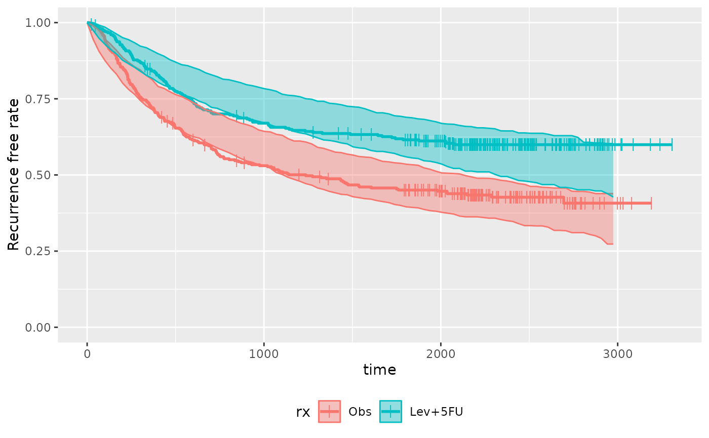
Or providing median survival summary table with
extract_medsurv_pi() function.
This functionality is only available for calc_km_pi()
output and has not been implemented for calc_ave_km_pi()
yet..
extract_medsurv_pi(km.pi)
#> # A tibble: 8 × 5
#>   rx          n description median quantile
#>   <fct>   <dbl> <chr>        <dbl>    <dbl>
#> 1 Obs       315 pi_low       1108.   0.0250
#> 2 Obs       315 pi_med       1538.   0.5
#> 3 Obs       315 pi_high      2113.   0.975
#> 4 Obs       315 obs          1236   NA
#> 5 Lev+5FU   304 pi_low       2126.   0.0250
#> 6 Lev+5FU   304 pi_med       2697.   0.5
#> 7 Lev+5FU   304 pi_high      2927.   0.975
#> 8 Lev+5FU   304 obs            NA   NA
Plot can also be made for subgroups.
You can see that prediction interval is wide for (depth: 1 & nodes4:
1) group, mainly due to small number of subjects
km.pi <- calc_km_pi(sim, trt = "rx", group = c("node4", "depth"))
#> Warning in calc_km_pi(sim, trt = "rx", group = c("node4", "depth")): 339 of 800
#> simulations (#rep * #trt * #group) did not reach median survival time and these
#> are not included for prediction interval calculation. You may want to delay the
#> `censor.dur` in simulation.

plot_km_pi(km.pi) +
  theme(legend.position = "bottom") +
  labs(y = "Recurrence free rate") +
  expand_limits(y = 0)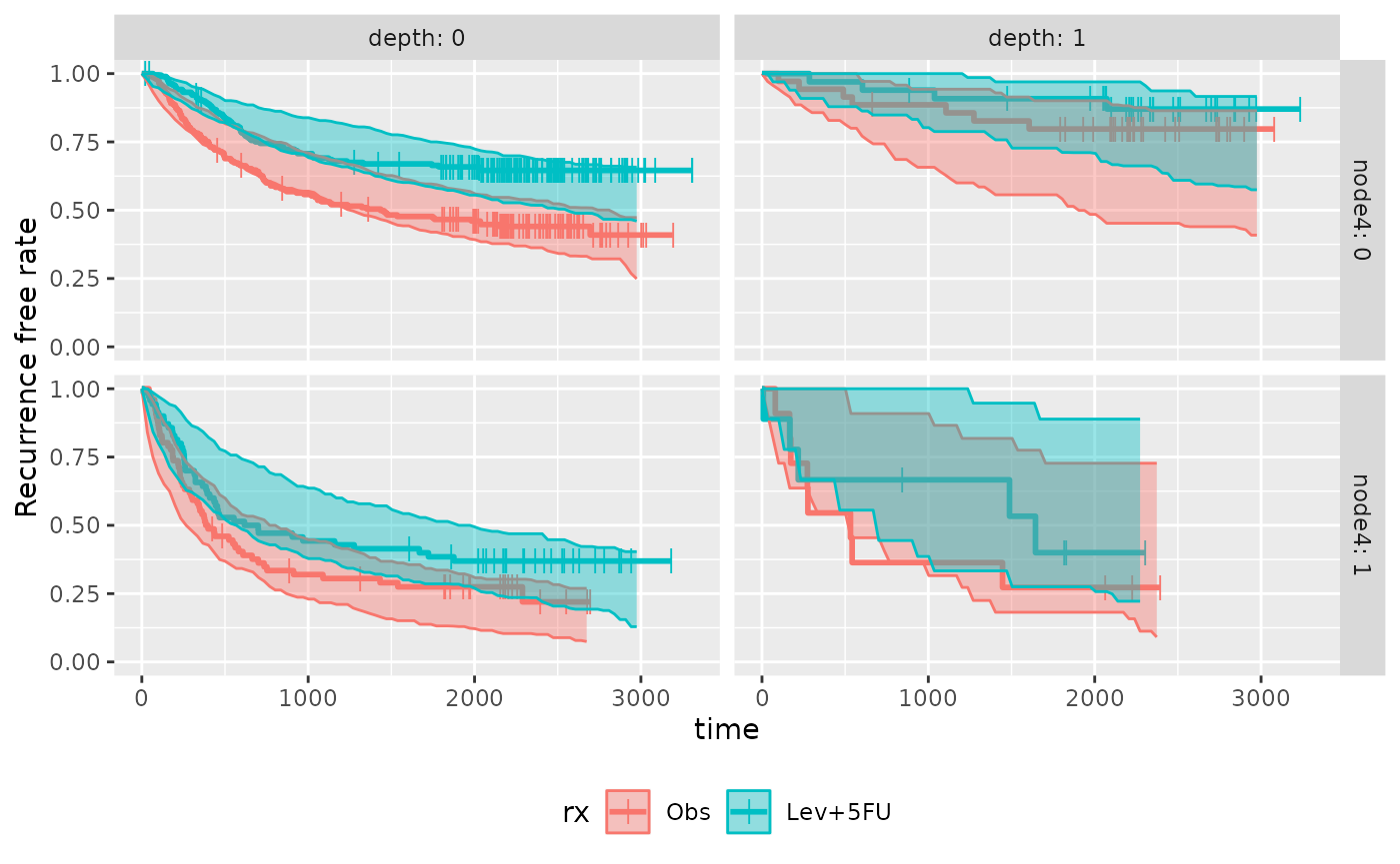
Hazard ratios (HRs)
To calculate prediction intervals of HRs,
calc_ave_hr_pi() or calc_hr_pi() can be used
on the simulated object above. Here I only generated subgroups based on
“depth”, since the very small N in (depth: 1 & nodes4: 1) can cause
issue with calculating HRs.
hr.pi <- calc_hr_pi(sim, trt = "rx", group = c("depth"))

hr.pi
#> ---- Simulated and observed (if calculated) hazard ratio ----
#> * Use `extract_hr_pi()` to extract prediction intervals and observed HR
#> * Use `extract_hr()` to extract individual simulated HRs
#> * Use `plot_hr_pi()` to draw histogram of predicted HR
#>
#> * Settings:
#>     trt: rx
#>          ('Lev+5FU' as test trt, 'Obs' as control)
#>     group: depth
#>     pi.range: 0.95
#>     calc.obs: TRUE
#>     method: Cox on simulated survival using `calc_hr_pi()`
plot_hr_pi(hr.pi)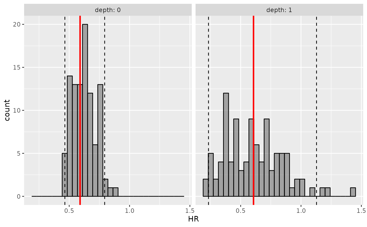
You can also extract prediction intervals and observed HR with
extract_hr_pi() function.
extract_hr_pi(hr.pi)
#> # A tibble: 8 × 5
#>   depth rx      description    HR quantile
#>   <dbl> <fct>   <chr>       <dbl>    <dbl>
#> 1     0 Lev+5FU pi_low      0.464   0.0250
#> 2     0 Lev+5FU pi_med      0.624   0.5
#> 3     0 Lev+5FU pi_high     0.794   0.975
#> 4     0 Lev+5FU obs         0.590  NA
#> 5     1 Lev+5FU pi_low      0.233   0.0250
#> 6     1 Lev+5FU pi_med      0.597   0.5
#> 7     1 Lev+5FU pi_high     1.13    0.975
#> 8     1 Lev+5FU obs         0.607  NA