![]()
The goal of survParamSim is to perform survival simulation with parametric survival model generated from ‘survreg’ function in ‘survival’ package. In each simulation, coefficients are resampled from variance-covariance matrix of parameter estimates, in order to capture uncertainty in model parameters.
Installation
You can install the package from CRAN.
install.packages("survParamSim")Alternatively, you can install the development version from GitHub.
# install.packages("devtools")
devtools::install_github("yoshidk6/survParamSim")
Example
This GitHub pages contains function references and vignette. The example below is a sneak peek of example outputs.
First, run survreg to fit parametric survival model:
library(dplyr)
#>
#> Attaching package: 'dplyr'
#> The following objects are masked from 'package:stats':
#>
#>     filter, lag
#> The following objects are masked from 'package:base':
#>
#>     intersect, setdiff, setequal, union
library(ggplot2)
library(survival)
library(survParamSim)
#> Warning: package 'survParamSim' was built under R version 4.2.3

set.seed(12345)

# ref for dataset https://vincentarelbundock.github.io/Rdatasets/doc/survival/colon.html
colon2 <-
  as_tibble(colon) %>%
  # recurrence only and not including Lev alone arm
  filter(rx != "Lev",
         etype == 1) %>%
  # Same definition as Lin et al, 1994
  mutate(rx = factor(rx, levels = c("Obs", "Lev+5FU")),
depth = as.numeric(extent <= 2))Next, run parametric bootstrap simulation:
sim <-
  surv_param_sim(object = fit.colon, newdata = colon2,
                 censor.dur = c(1800, 3000),
                 # Simulating only 100 times to make the example go fast
                 n.rep = 100)

sim
#> ---- Simulated survival data with the following model ----
#> survreg(formula = Surv(time, status) ~ rx + node4 + depth, data = colon2,
#>     dist = "lognormal")
#>
#> * Use `extract_sim()` function to extract individual simulated survivals
#> * Use `calc_km_pi()` function to get survival curves and median survival time
#> * Use `calc_hr_pi()` function to get hazard ratio
#>
#> * Settings:
#>     #simulations: 100
#>     #subjects: 619 (without NA in model variables)
Calculate survival curves with prediction intervals:
km.pi <- calc_km_pi(sim, trt = "rx", group = c("node4", "depth"))
#> Warning in calc_km_pi(sim, trt = "rx", group = c("node4", "depth")): 339 of 800
#> simulations (#rep * #trt * #group) did not reach median survival time and these
#> are not included for prediction interval calculation. You may want to delay the
#> `censor.dur` in simulation.

km.pi
#> ---- Simulated and observed (if calculated) survival curves ----
#> * Use `extract_medsurv_pi()` to extract prediction intervals of median survival times
#> * Use `extract_km_pi()` to extract prediction intervals of K-M curves
#> * Use `plot_km_pi()` to draw survival curves
#>
#> * Settings:
#>     trt: rx
#>     group: node4
#>     pi.range: 0.95
#>     calc.obs: TRUE
plot_km_pi(km.pi) +
  theme(legend.position = "bottom") +
  labs(y = "Recurrence free rate") +
  expand_limits(y = 0)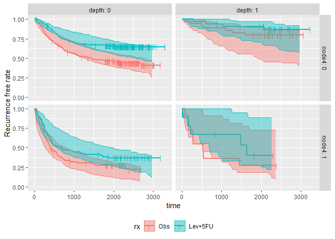
extract_medsurv_pi(km.pi) # Not implemented for calc_ave_km_pi yet; available for calc_km_pi
#> # A tibble: 32 × 7
#>    node4 depth rx          n description median quantile
#>    <dbl> <dbl> <fct>   <dbl> <chr>        <dbl>    <dbl>
#>  1     0     0 Obs       193 pi_low       1257.   0.0250
#>  2     0     0 Obs       193 pi_med       1895.   0.5
#>  3     0     0 Obs       193 pi_high      2713.   0.975
#>  4     0     0 Obs       193 obs          1436   NA
#>  5     0     0 Lev+5FU   192 pi_low       2429.   0.0250
#>  6     0     0 Lev+5FU   192 pi_med       2716.   0.5
#>  7     0     0 Lev+5FU   192 pi_high      2908.   0.975
#>  8     0     0 Lev+5FU   192 obs            NA   NA
#>  9     0     1 Obs        35 pi_low       1539.   0.0250
#> 10     0     1 Obs        35 pi_med       2558.   0.5
#> # … with 22 more rows
Calculate hazard ratios with prediction intervals:
hr.pi <- calc_hr_pi(sim, trt = "rx", group = c("depth"))

hr.pi
#> ---- Simulated and observed (if calculated) hazard ratio ----
#> * Use `extract_hr_pi()` to extract prediction intervals and observed HR
#> * Use `extract_hr()` to extract individual simulated HRs
#> * Use `plot_hr_pi()` to draw histogram of predicted HR
#>
#> * Settings:
#>     trt: rx
#>          ('Lev+5FU' as test trt, 'Obs' as control)
#>     group: depth
#>     pi.range: 0.95
#>     calc.obs: TRUE
plot_hr_pi(hr.pi)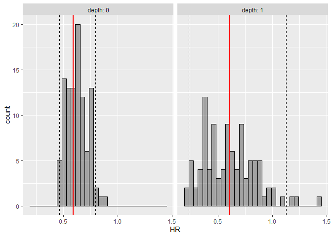
extract_hr_pi(hr.pi)
#> # A tibble: 8 × 5
#>   depth rx      description    HR quantile
#>   <dbl> <fct>   <chr>       <dbl>    <dbl>
#> 1     0 Lev+5FU pi_low      0.464   0.0250
#> 2     0 Lev+5FU pi_med      0.624   0.5
#> 3     0 Lev+5FU pi_high     0.794   0.975
#> 4     0 Lev+5FU obs         0.590  NA
#> 5     1 Lev+5FU pi_low      0.233   0.0250
#> 6     1 Lev+5FU pi_med      0.597   0.5
#> 7     1 Lev+5FU pi_high     1.13    0.975
#> 8     1 Lev+5FU obs         0.607  NA